A simple BLDC speed control by SimuLink

Chao, Chun-Tang (»¯¬K´Å) in STUST

2015.11.21

² BLDC Model (with Driver)
I/P: Duty Cycle ( 0~1 OR 0% ~100% )
O/P: Rotation Speed

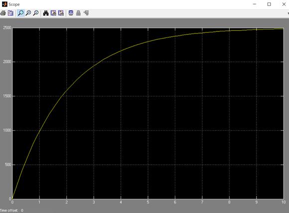
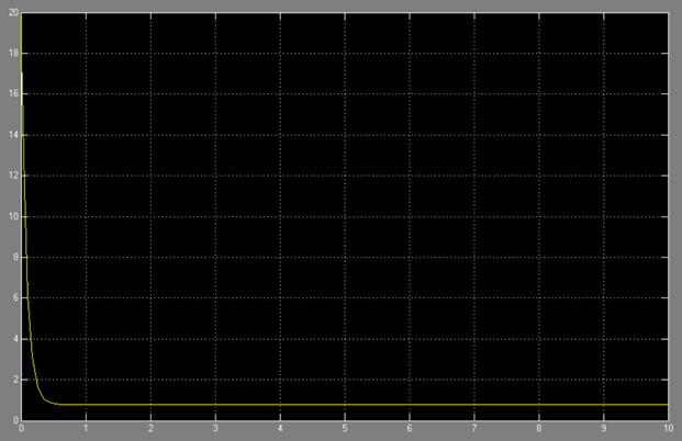
The above unit-step response (time constant = 2s) may imply that
Duty Cycle = 100% => Rotation Speed = 2500 rpm

Duty Cycle = 90% => Rotation Speed = 2500X0.9= 2250 rpm

Duty Cycle = 80% => Rotation Speed = 2500X0.8= 2000 rpm

¡K¡K¡K¡K¡K¡K¡K¡K¡K¡K¡K¡K¡K¡K¡K¡K¡K¡K¡K¡K¡K..

The above simulation can also be regarded as the open-loop control (BLDC_open.mdl).

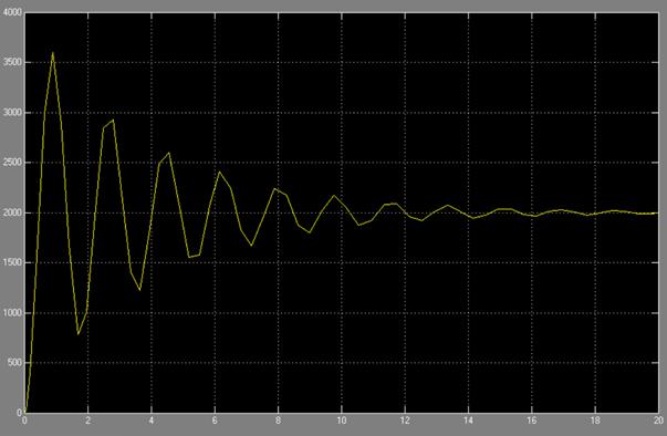
² BLDC closed-loop control ¡V with P controller (Kp = 0.01) (BLDC_closed_P.mdl)

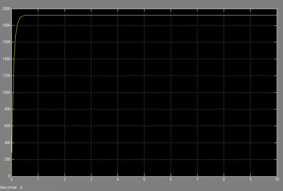
System I/P: Desired rotation speed= 2000 rpm

System O/P: Rotation Speed (steady-state) = rpm Note: e_ss (steady-state error) = 2000-1923 = 77 rpm

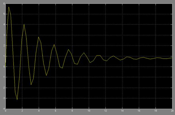
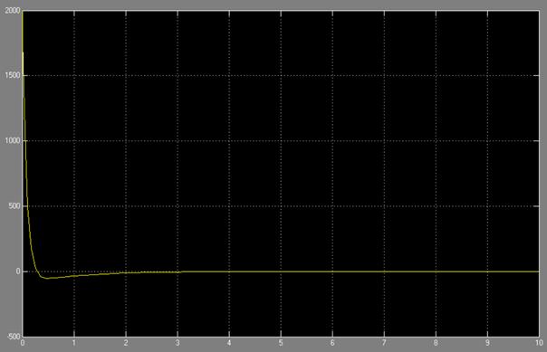
Error Signal (Controller I/P): The following figure also shows e_ss (steady-state error) = 2000-1923 ~= 77 rpm

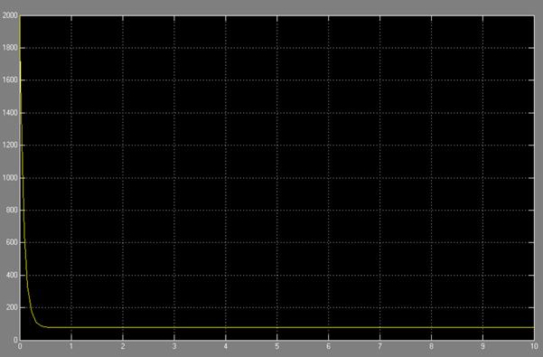
Controller O/P: When the steady-state is achieved, the controller output is 0.77, which means the final duty-cycle command to the BLDC will be 77%.

Remark: With closed-loop P controller, we find that the system time constant is greatly reduced, which yields much faster response. The crucial drawback is the steady-state error, which can be eliminated by the following I controller.

In the initial period 0~0.3s, the duty-cycle command to the BLDC is almost greater than 1 (100%), which is nonsense! Do you find it?
I hope this example can show you the difference between practical implementation and theoretical simulation.

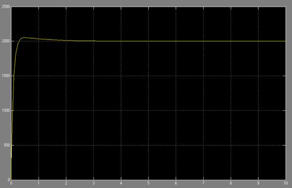
² BLDC closed-loop control ¡V with I controller (KI = 0.01) (BLDC_closed_I.mdl)

System I/P: Desired rotation speed= 2000 rpm

System O/P: Rotation Speed (steady-state) = 2000 rpm Note: e_ss (steady-state error) = 0

Error Signal (Controller I/P): The following figure also shows e_ss (steady-state error) = 0 rpm

Controller O/P: When the steady-state is achieved, the controller output is 0.8, which means the final duty-cycle command to the BLDC will be 80%.

Remark: The I controller successfully make e_ss approach to zero.

In the beginning BLDC model, we have ¡§Duty Cycle = 80% => Rotation Speed = 2500X0.8= 2000 rpm¡¨. That¡¦s why the final duty-cycle command to the BLDC will be 80%.

In this case, the duty-cycle command to the BLDC is also usually greater than 1 (100%), thus the practical result will be different.

² BLDC closed-loop control ¡V with PI controller (Kp=0.01 and KI = 0.01) (BLDC_closed_P_I.mdl)

System I/P: Desired rotation speed= 2000 rpm

System O/P: Rotation Speed (steady-state) = 2000 rpm Note: e_ss (steady-state error) = 0

Error Signal (Controller I/P): The following figure also shows e_ss (steady-state error) = 0 rpm

Controller O/P: When the steady-state is achieved, the controller output is 0.8, which means the final duty-cycle command to the BLDC will be 80%.

Remark: The PI controller has both advantages of P controller and I controller. The system response is much faster and the steady-state error can be eliminated to be zero. In the initial period 0~0.3s, the duty-cycle command to the BLDC is also greater than 1 (100%), thus the above simulation result will not be the same as the practical result. In fact, the BLDC is often controlled by micro-controller. To increase the accuracy, you may apply the digital control theory and consider the sampling time.

You must already find both in the open-loop control and the closed-loop control with I or PI controller, the final duty-cycle command to the BLDC is 80%, the same value, to keep rotation speed at 2000 rpm. But the closed-loop control system has many advantages over the open-loop control system.

This web-page just hopes to show you the importance of theory and the difference between practical implementation and theoretical simulation.

Happy Learning !